Use cttab in the Analysis

What this Document Does

The package cctu has been updated to utilize the DLU file and CLU file to facilitate the analyzing process. The newly added functions will not affect previous process. But here, in this document we are going to learn some new functions provided in the package to facilitate your analysis. Before you start, you should get yourself familiarized with the cctu package by looking through the Analysis Template vignette. Remember, the sumby function will not benefit from any of the data attribute related new functions mentioned in this document. Namely, the variable label and value labels will not have an effect on the output. You don’t need to go through everything in this document if you are going to stick to the sumby function.

What’s new

Variable and value label

If you are familiar with SAS, Stata or SPSS, you should already know there’s a variable label and value label (variable format in some). The variable label gives you the description of the variable, and the value label is to explain what the values stand for. The variable will stay as a numeric but has categories attached to it. Which means, you can subset or manipulate it like a numerical variable but report the data as a categorical one. It is important to understand this, let’s use mtcars dataset and demonstrate how it works.

data(mtcars)
# Assign variable label
var_lab(mtcars$am) <- "Transmission"

# Assign value label with named vector
val_lab(mtcars$am) <- c("Automatic" = 0, "Manual" = 1)
str(mtcars$am)
#>  num [1:32] 1 1 1 0 0 0 0 0 0 0 ...
#>  - attr(*, "label")= chr "Transmission"
#>  - attr(*, "labels")= Named num [1:2] 0 1
#>   ..- attr(*, "names")= chr [1:2] "Automatic" "Manual"

As you can above, label and labels attributes were added. But the variable is numeric. You can still summarize it as numeric variable as below:

summary(mtcars$am)
#>    Min. 1st Qu.  Median    Mean 3rd Qu.    Max. 
#>  0.0000  0.0000  0.0000  0.4062  1.0000  1.0000

You can convert the value label to factor just before your final analysis. The to_factor function replace the value with labels and convert the variable to factor.

# Extract variable label
var_lab(mtcars$am)
#> [1] "Transmission"

# Convert variable to factor with labels attached to it
table(to_factor(mtcars$am))
#> 
#> Automatic    Manual 
#>        19        13

But be cautious, some R process might drop the variable or value label attributes. Normally it won’t, but you should check it before report if you are not sure. For example, as.numeric, as.character and as.logiac will drop the variable and value label. There are to_numeric, to_character and to_logical can be used to convert the data type. You can also use the copy_lab function to copy the variable and value labels from the other variable.

You can use var_lab to extract the variable label or assign one. And use has_label to check if the variable has any variable label with it. You may also want to use drop_lab to drop the variable label.

For value label, you can use val_lab to extract or assign value label. And use has_labels to check if the variable has a value label. There are also unval function to drop the value label and lab2val to replace the data.frame value to its corresponding value labels.

MACRO dataset utility functions

There are new functions have been added to utilize the DLU and CLU files for the data analysis. The apply_macro_dict function uses DLU and CLU file to assign variable and value labels to the dataset. This function will convert the variable name in the data and DLU to lower case by default. This will also convert the dataset based on the variable type as in the DLU file. If you don’t want to convert the variable name to lower cases, you should set clean_names = FALSE.

The extract_form can extract MACRO data by form and visits. The data will be converted to data.table class, which is an extension of the data.frame and works exactly the same. It is a great package with lots of data manipulation capability, you should seek the website for more details. But one thing to remember is that all the names in the variable selection will be considered as a variable of the data.

vars <- c("mpg", "am")
# You can do this in the normal data.frame
mtcars[, vars]

# But you can't do this for the data.table
dat <- data.table::data.table(mtcars)
mtcars[, vars]

# You need to add with=FALSE to do that
mtcars[, vars, with = FALSE]

Table function

You might already knew how to use the sumby function, but now a new function called cttab has been added. The difference between these two functions are the latter can handle variable label and value labels. You can feed the labelled data to this function and it will populate a summary table. Report data by treatment group, stratify tables by visit. Also, you can report variable based on some conditions and group the variable in the report. It generates a missing report internally and you can dump the missing report at the end. No extra step is needed. It will also produce the summary plots of the variables. The produced plots will be arrange to 3 by 3 and new plot will be producd if the variables exceeds 9. The remaining of this document will show you with a working case.

Setting options

The cctab function has a good flexibility, which means it has lots of parameters you can use. You should check out the manual of the cctab function. But, you can use options to set the default value of the parameters to be used by cctab. Below is setting some of the options, for more details please check out the cctab function manuals.

options(cctu_digits = 3) # keep 3 digits for numerical value
options(cctu_digits_pct = 0) # keep 0 digits for percentage
options(cctu_subjid_string = "subjid") # Set subject ID string
options(cctu_print_plot = FALSE) # Don't produce plots

Working example

In this section, we will show how to populate tables.

Data reading

Usual case

You should read the data as before, but you can and should read the data by setting all the columns to character. This will be handled later. Same process can be found in the Analysis Template vignette.

# Read example data
dt <- read.csv(system.file("extdata", "pilotdata.csv", package = "cctu"), colClasses = "character")

# Read DLU and CLU
dlu <- read.csv(system.file("extdata", "pilotdata_dlu.csv", package = "cctu"))
clu <- read.csv(system.file("extdata", "pilotdata_clu.csv", package = "cctu"))

Vertically splited multiple data

If you have multiple datasets, you should combine them at this stage. If multiple datasets are given and they have the same variable name, you can use rbind function to combine data together. If you have different datasets with different variable names except for some key variables, you can use merge_data function to combine them together.

# Read example data
dt_a <- read.csv(system.file("extdata", "test_A.csv", package = "cctu"),
  colClasses = "character"
)
dt_b <- read.csv(system.file("extdata", "test_B.csv", package = "cctu"),
  colClasses = "character"
)

# Read DLU and CLU
dlu_a <- read.csv(system.file("extdata", "test_A_DLU.csv", package = "cctu"))
dlu_b <- read.csv(system.file("extdata", "test_B_DLU.csv", package = "cctu"))
clu_a <- read.csv(system.file("extdata", "test_A_CLU.csv", package = "cctu"))
clu_b <- read.csv(system.file("extdata", "test_B_CLU.csv", package = "cctu"))

# Merge dataset with merge_data function
res <- merge_data(
  datalist = list(dt_a, dt_b), dlulist = list(dlu_a, dlu_b),
  clulist = list(clu_a, clu_b)
)
dt <- res$data # Extract combined data
dlu <- res$dlu # Extract combined DLU data
clu <- res$clu # Extract combined CLU data

Apply macro dictionary

Next, we will apply the DLU and CLU files to the dataset. Do not clean variable name in the dataset and DLU/CLU files before applying apply_macro_dict. The function can handle variable name cleaning by setting clean_names = TRUE, this is default behaviour. The apply_macro_dict function will clean the variable name in the DLU and CLU, then apply these macro meta data to the target dataset. The cleaned DLU data will be sotred internally and is further used by cttab to report missingness. You can use get_dlu to extract the internal DLU data after applying apply_macro_dict to the dataset for further useage or as a reference. Although you can use set_dlu to change the internal DLU data stored by apply_macro_dict, this is not recommended unless you know what you are doing. This will have an impact on the missing report.

# Create subjid
dt$subjid <- substr(dt$USUBJID, 8, 11)

# Apply CLU and DLU files
dt <- apply_macro_dict(dt, dlu = dlu, clu = clu, clean_names = FALSE)

# Give new variable a label
var_lab(dt$subjid) <- "Subject ID"

After this, you should follow the Analysis Template vignette and setup the population etc.

Next we will do some data analysis.

Data analysis

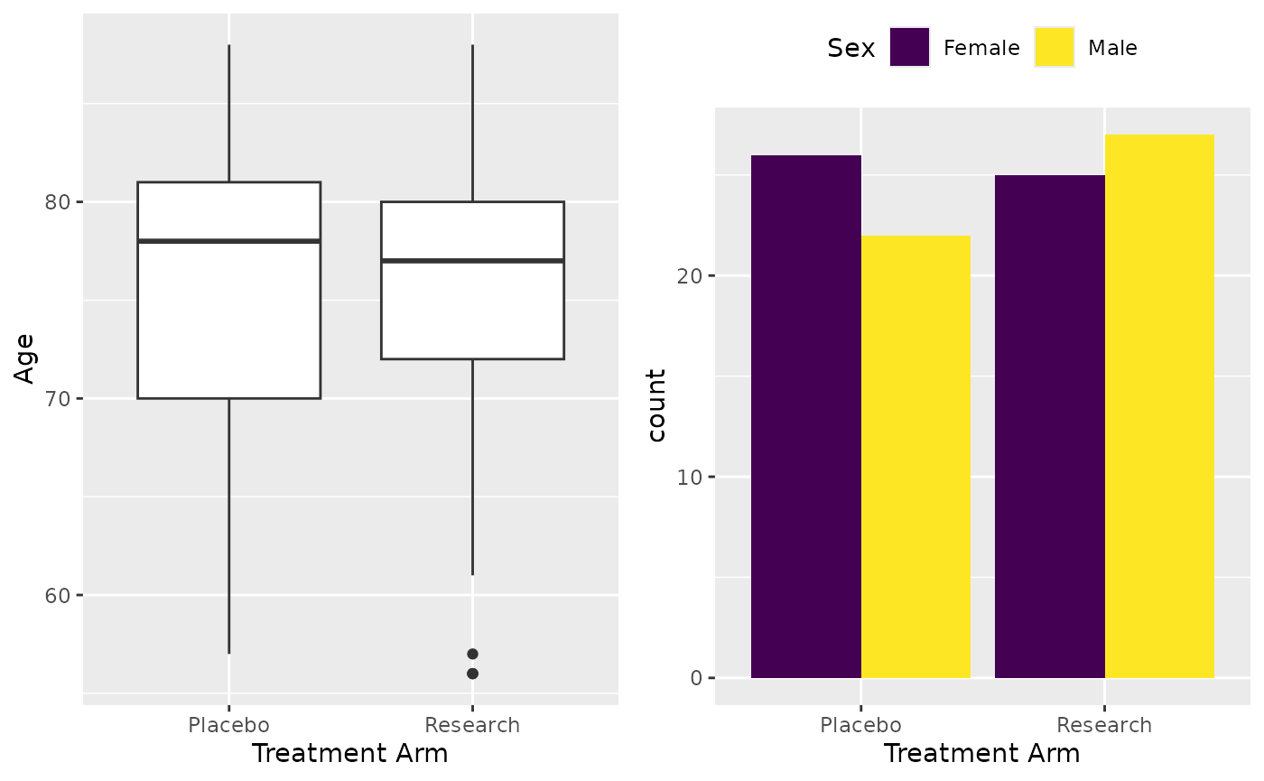
After you have attached the population, next thing you may want to do is extract a particular form from the data. For the table, assume we are reporting age, sex and BMI from the patient registration form by treatment arm. For demonstrating the filtering, we only report non-white patients’ BMI.

# Attach population
attach_pop("1.1")

# Extract patient patient registration form and keep subjid variable
df <- extract_form(dt, "PatientReg", vars_keep = c("subjid"))

# Now report Age, Sex and BMI. For BMI, report not white only
X <- cttab(
  x = c("AGE", "SEX", "BMIBL"), # Variable to report
  group = "ARM", # Group variable
  data = df, # Data
  select = c("BMIBL" = "RACEN != 1")
) # Filter for variable BMI


# Write table
X
#> ┌───────────────────┬─────────────────┬─────────────────┬─────────────────┐
#> |                   │     Placebo     │    Research     │      Total      |
#> ├───────────────────┴─────────────────┴─────────────────┴─────────────────┤
#> |Observation        │       48        │       52        │       100       |
#> ├───────────────────┬─────────────────┬─────────────────┬─────────────────┤
#> ├───────────────────┴─────────────────┴─────────────────┴─────────────────┤
#> |Age                                                                      |
#> ├───────────────────┬─────────────────┬─────────────────┬─────────────────┤
#> |  Valid Obs.       │       48        │       52        │       100       |
#> |  Mean (SD)        │   75.5 (7.86)   │   74.8 (8.04)   │   75.1 (7.93)   |
#> |  Median [Min, Max]│78.0 [57.0, 88.0]│77.0 [56.0, 88.0]│77.0 [56.0, 88.0]|
#> ├───────────────────┴─────────────────┴─────────────────┴─────────────────┤
#> |Sex                                                                      |
#> ├───────────────────┬─────────────────┬─────────────────┬─────────────────┤
#> |  Female           │   26/48 (54%)   │   25/52 (48%)   │  51/100 (51%)   |
#> |  Male             │   22/48 (46%)   │   27/52 (52%)   │  49/100 (49%)   |
#> ├───────────────────┴─────────────────┴─────────────────┴─────────────────┤
#> |Baseline BMI (kg/m^2)                                                    |
#> ├───────────────────┬─────────────────┬─────────────────┬─────────────────┤
#> |  Valid Obs.       │        5        │        6        │       11        |
#> |  Mean (SD)        │   27.8 (3.98)   │   24.6 (3.54)   │   26.0 (3.93)   |
#> |  Median [Min, Max]│27.9 [23.4, 32.8]│23.5 [21.3, 31.4]│24.3 [21.3, 32.8]|
#> └───────────────────┴─────────────────┴─────────────────┴─────────────────┘

Formula interface

One can use formula in the cctab just like lm, but you will not be able to group variables (described in the later section). The left hand side of the formula is the variables to be summarised. Right hand side of the formula is the grouping and/or row splitting variables. The by visit variable should be separated by | with grouping variable, use 1 if there is no grouping variables. No group or row_split parameters to be used in the formula interface. All the other parameters are the same.

# No grouping
X <- cttab(AGE + SEX + BMIBL ~ 1, data = df)
# Group summarise by ARM
X <- cttab(AGE + SEX + BMIBL ~ ARM, data = df)
# Group summarise by ARM and split by visit cycle
X <- cttab(AST + BILI ~ ARM | AVISIT, data = df)
# Split by visit cycle
X <- cttab(AST + BILI ~ 1 | AVISIT, data = df)

Missing data report

The cttab function will report the missing internally. You can use the following to get the missing report.

# This will save the missing report under Output folder
# Or you can set the output folder and name
dump_missing_report()

# Pull out the missing report if you want
miss_rep <- get_missing_report()

# Reset missing report
reset_missing_report()

After this, you can finish the remaining as in the Analysis Template vignette.

More to cttab

As you have seen previously, the cttab function can easily populate simple tables.

Simple table

Table only some variables, no treatment arm or variable selection.

X <- cttab(
  x = c("AGE", "SEX", "BMIBL"), # Variable to report
  data = df
) # Data


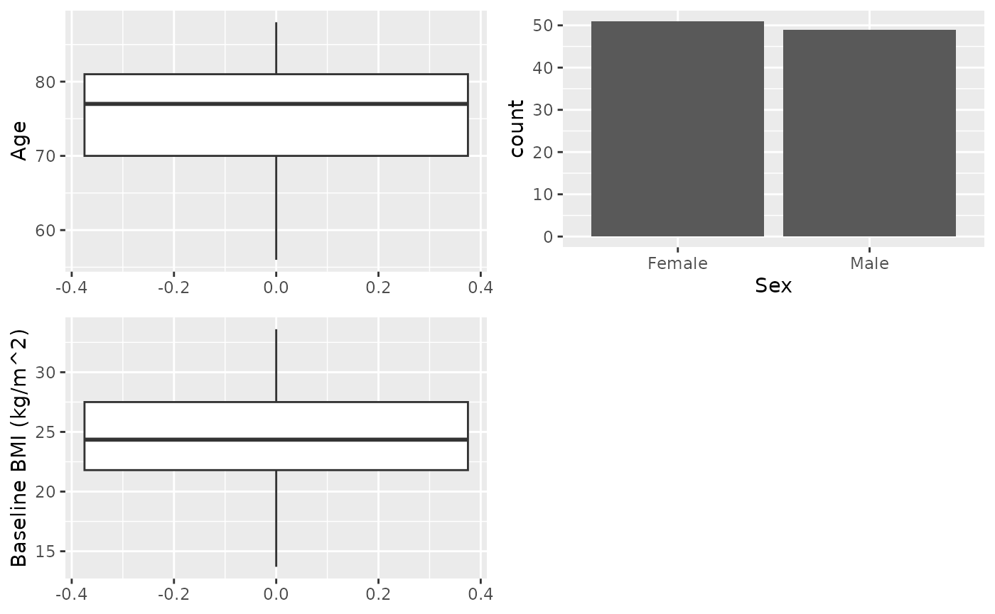
X
#> ┌───────────────────┬─────────────────┐
#> |                   │      Total      |
#> ├───────────────────┴─────────────────┤
#> |Age                                  |
#> ├───────────────────┬─────────────────┤
#> |  Valid Obs.       │       100       |
#> |  Mean (SD)        │   75.1 (7.93)   |
#> |  Median [Min, Max]│77.0 [56.0, 88.0]|
#> ├───────────────────┴─────────────────┤
#> |Sex                                  |
#> ├───────────────────┬─────────────────┤
#> |  Female           │  51/100 (51%)   |
#> |  Male             │  49/100 (49%)   |
#> ├───────────────────┴─────────────────┤
#> |Baseline BMI (kg/m^2)                |
#> ├───────────────────┬─────────────────┤
#> |  Valid Obs.       │       100       |
#> |  Mean (SD)        │   24.5 (4.15)   |
#> |  Median [Min, Max]│24.4 [13.7, 33.6]|
#> └───────────────────┴─────────────────┘

By group and filter

This is what we have seen before

X <- cttab(
  x = c("AGE", "SEX", "BMIBL"), # Variable to report
  group = "ARM", # Group variable
  data = df, # Data
  select = c("BMIBL" = "RACEN != 1")
) # Filter for variable BMI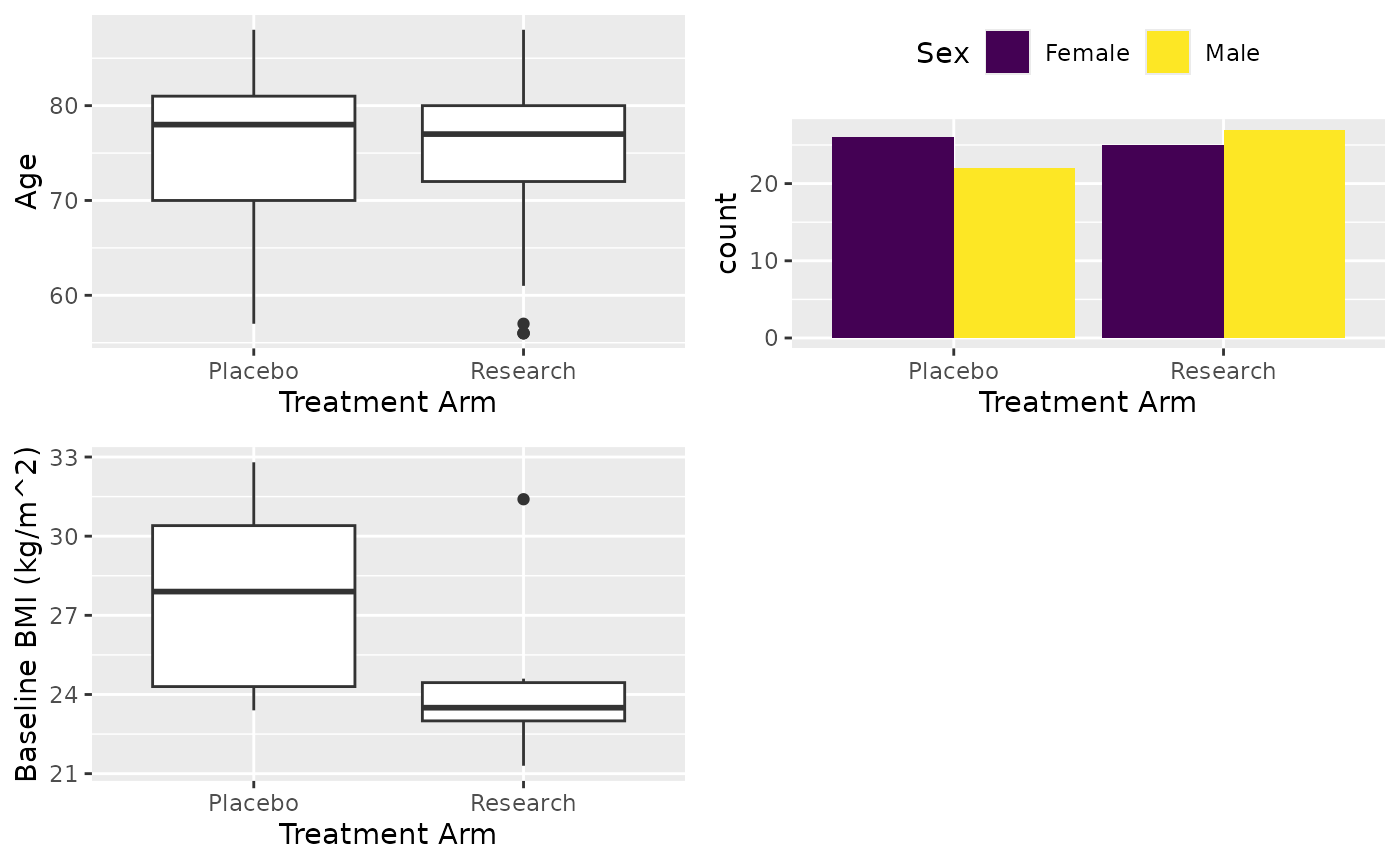


X
#> ┌───────────────────┬─────────────────┬─────────────────┬─────────────────┐
#> |                   │     Placebo     │    Research     │      Total      |
#> ├───────────────────┴─────────────────┴─────────────────┴─────────────────┤
#> |Observation        │       48        │       52        │       100       |
#> ├───────────────────┬─────────────────┬─────────────────┬─────────────────┤
#> ├───────────────────┴─────────────────┴─────────────────┴─────────────────┤
#> |Age                                                                      |
#> ├───────────────────┬─────────────────┬─────────────────┬─────────────────┤
#> |  Valid Obs.       │       48        │       52        │       100       |
#> |  Mean (SD)        │   75.5 (7.86)   │   74.8 (8.04)   │   75.1 (7.93)   |
#> |  Median [Min, Max]│78.0 [57.0, 88.0]│77.0 [56.0, 88.0]│77.0 [56.0, 88.0]|
#> ├───────────────────┴─────────────────┴─────────────────┴─────────────────┤
#> |Sex                                                                      |
#> ├───────────────────┬─────────────────┬─────────────────┬─────────────────┤
#> |  Female           │   26/48 (54%)   │   25/52 (48%)   │  51/100 (51%)   |
#> |  Male             │   22/48 (46%)   │   27/52 (52%)   │  49/100 (49%)   |
#> ├───────────────────┴─────────────────┴─────────────────┴─────────────────┤
#> |Baseline BMI (kg/m^2)                                                    |
#> ├───────────────────┬─────────────────┬─────────────────┬─────────────────┤
#> |  Valid Obs.       │        5        │        6        │       11        |
#> |  Mean (SD)        │   27.8 (3.98)   │   24.6 (3.54)   │   26.0 (3.93)   |
#> |  Median [Min, Max]│27.9 [23.4, 32.8]│23.5 [21.3, 31.4]│24.3 [21.3, 32.8]|
#> └───────────────────┴─────────────────┴─────────────────┴─────────────────┘

Split table row by visit

You can define row_split parameter to the name of visit or repeat variable.

attach_pop("1.1")
df <- extract_form(dt, "Lab", vars_keep = c("subjid", "ARM"))

X <- cttab(
  x = c("AST", "BILI", "ALT"),
  group = "ARM",
  data = df,
  row_split = "AVISIT", # Visit variable
  select = c("ALT" = "PERF == 1")
)


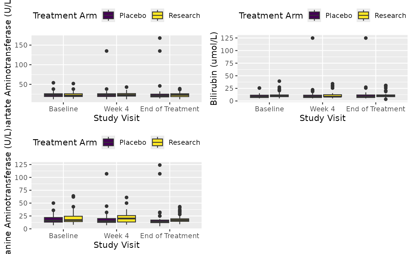
X
#> ┌───────────────────┬─────────────────┬─────────────────┬─────────────────┐
#> |                   │     Placebo     │    Research     │      Total      |
#> ├───────────────────┴─────────────────┴─────────────────┴─────────────────┤
#> |Study Visit = Baseline                                                   |
#> ├───────────────────┬─────────────────┬─────────────────┬─────────────────┤
#> |Observation        │       48        │       52        │       100       |
#> ├───────────────────┴─────────────────┴─────────────────┴─────────────────┤
#> |Aspartate Aminotransferase (U/L)                                         |
#> ├───────────────────┬─────────────────┬─────────────────┬─────────────────┤
#> |  Valid Obs.       │       47        │       52        │       99        |
#> |  Mean (SD)        │   23.4 (7.09)   │   23.6 (7.05)   │   23.5 (7.04)   |
#> |  Median [Min, Max]│23.0 [12.0, 54.0]│21.5 [13.0, 52.0]│23.0 [12.0, 54.0]|
#> |  Missing          │     1 (2%)      │                 │     1 (1%)      |
#> ├───────────────────┴─────────────────┴─────────────────┴─────────────────┤
#> |Bilirubin (umol/L)                                                       |
#> ├───────────────────┬─────────────────┬─────────────────┬─────────────────┤
#> |  Valid Obs.       │       46        │       51        │       97        |
#> |  Mean (SD)        │   10.0 (4.38)   │   11.4 (6.01)   │   10.8 (5.32)   |
#> |  Median [Min, Max]│8.55 [5.13, 25.7]│10.3 [5.13, 39.3]│10.3 [5.13, 39.3]|
#> |  Missing          │     2 (4%)      │     1 (2%)      │     3 (3%)      |
#> ├───────────────────┴─────────────────┴─────────────────┴─────────────────┤
#> |Alanine Aminotransferase (U/L)                                           |
#> ├───────────────────┬─────────────────┬─────────────────┬─────────────────┤
#> |  Valid Obs.       │       45        │       40        │       85        |
#> |  Mean (SD)        │   18.1 (8.01)   │   22.1 (13.2)   │   20.0 (10.9)   |
#> |  Median [Min, Max]│16.0 [7.00, 50.0]│17.0 [8.00, 64.0]│16.0 [7.00, 64.0]|
#> |  Missing          │                 │     2 (5%)      │     2 (2%)      |
#> ├───────────────────┴─────────────────┴─────────────────┴─────────────────┤
#> |Study Visit = Week 4                                                     |
#> ├───────────────────┬─────────────────┬─────────────────┬─────────────────┤
#> |Observation        │       43        │       44        │       87        |
#> ├───────────────────┴─────────────────┴─────────────────┴─────────────────┤
#> |Aspartate Aminotransferase (U/L)                                         |
#> ├───────────────────┬─────────────────┬─────────────────┬─────────────────┤
#> |  Valid Obs.       │       41        │       43        │       84        |
#> |  Mean (SD)        │   25.1 (18.4)   │   23.8 (6.39)   │   24.4 (13.6)   |
#> |  Median [Min, Max]│23.0 [12.0, 135] │23.0 [12.0, 43.0]│23.0 [12.0, 135] |
#> |  Missing          │     2 (5%)      │     1 (2%)      │     3 (3%)      |
#> ├───────────────────┴─────────────────┴─────────────────┴─────────────────┤
#> |Bilirubin (umol/L)                                                       |
#> ├───────────────────┬─────────────────┬─────────────────┬─────────────────┤
#> |  Valid Obs.       │       42        │       44        │       86        |
#> |  Mean (SD)        │   12.7 (18.2)   │   11.4 (6.51)   │   12.0 (13.5)   |
#> |  Median [Min, Max]│8.55 [5.13, 125] │8.55 [5.13, 34.2]│8.55 [5.13, 125] |
#> |  Missing          │     1 (2%)      │                 │     1 (1%)      |
#> ├───────────────────┴─────────────────┴─────────────────┴─────────────────┤
#> |Alanine Aminotransferase (U/L)                                           |
#> ├───────────────────┬─────────────────┬─────────────────┬─────────────────┤
#> |  Valid Obs.       │       39        │       38        │       77        |
#> |  Mean (SD)        │   18.9 (16.1)   │   21.6 (11.0)   │   20.2 (13.8)   |
#> |  Median [Min, Max]│15.0 [7.00, 107] │20.0 [8.00, 61.0]│16.0 [7.00, 107] |
#> |  Missing          │                 │     3 (7%)      │     3 (4%)      |
#> ├───────────────────┴─────────────────┴─────────────────┴─────────────────┤
#> |Study Visit = End of Treatment                                           |
#> ├───────────────────┬─────────────────┬─────────────────┬─────────────────┤
#> |Observation        │       47        │       50        │       97        |
#> ├───────────────────┴─────────────────┴─────────────────┴─────────────────┤
#> |Aspartate Aminotransferase (U/L)                                         |
#> ├───────────────────┬─────────────────┬─────────────────┬─────────────────┤
#> |  Valid Obs.       │       45        │       48        │       93        |
#> |  Mean (SD)        │   27.4 (27.9)   │   23.1 (6.04)   │   25.2 (19.9)   |
#> |  Median [Min, Max]│21.0 [14.0, 168] │23.0 [12.0, 39.0]│22.0 [12.0, 168] |
#> |  Missing          │     2 (4%)      │     2 (4%)      │     4 (4%)      |
#> ├───────────────────┴─────────────────┴─────────────────┴─────────────────┤
#> |Bilirubin (umol/L)                                                       |
#> ├───────────────────┬─────────────────┬─────────────────┬─────────────────┤
#> |  Valid Obs.       │       45        │       46        │       91        |
#> |  Mean (SD)        │   12.5 (17.7)   │   11.5 (6.39)   │   12.0 (13.2)   |
#> |  Median [Min, Max]│8.55 [5.13, 125] │10.3 [3.42, 30.8]│8.55 [3.42, 125] |
#> |  Missing          │     2 (4%)      │     4 (8%)      │     6 (6%)      |
#> ├───────────────────┴─────────────────┴─────────────────┴─────────────────┤
#> |Alanine Aminotransferase (U/L)                                           |
#> ├───────────────────┬─────────────────┬─────────────────┬─────────────────┤
#> |  Valid Obs.       │       45        │       43        │       88        |
#> |  Mean (SD)        │   19.6 (21.8)   │   19.7 (8.41)   │   19.6 (16.6)   |
#> |  Median [Min, Max]│14.0 [5.00, 124] │17.0 [9.00, 43.0]│16.0 [5.00, 124] |
#> |  Missing          │                 │     1 (2%)      │     1 (1%)      |
#> └───────────────────┴─────────────────┴─────────────────┴─────────────────┘

Group variable

In this example, we will report demographic variable, lab results and lab abnormality. Variables will be grouped, no group name will be given to demographic variables, “Blood” to lab results and “Pts with Abnormal” to lab abnormality. Here, we count the number of patients with abnormal lab results. The cttab will report the count and percentage of TRUE. This is useful if you want to report patient numbers for different condition that belong to one category. Below is how to do it:

# Prepare data as before
attach_pop("1.1")
df <- extract_form(dt, "PatientReg", vars_keep = c("subjid"))
base_lab <- extract_form(dt, "Lab",
  visit = "SCREENING",
  vars_keep = c("subjid")
)

# Define abnormal
base_lab$ABNORMALT <- base_lab$ALT > 22.5
var_lab(base_lab$ABNORMALT) <- "ALT abnormal"
base_lab$ABNORMAST <- base_lab$AST > 25.5
var_lab(base_lab$ABNORMAST) <- "AST abnormal"

df <- merge(df, base_lab, by = "subjid")

# Table
X <- cttab(
  x = list(c("AGE", "SEX", "BMIBL"),
    # Group lab variable
    "Blood" = c("ALT", "AST"),
    # Group abnormal variable
    "Pts with Abnormal" = c("ABNORMAST", "ABNORMALT")
  ),
  group = "ARM",
  data = df,
  # Add some filtering
  select = c(
    "BMIBL" = "RACEN != 1",
    "ALT" = "PERF == 1"
  )
)


X
#> ┌───────────────────┬─────────────────┬─────────────────┬─────────────────┐
#> |                   │     Placebo     │    Research     │      Total      |
#> ├───────────────────┴─────────────────┴─────────────────┴─────────────────┤
#> |Observation        │       48        │       52        │       100       |
#> ├───────────────────┬─────────────────┬─────────────────┬─────────────────┤
#> ├───────────────────┴─────────────────┴─────────────────┴─────────────────┤
#> |Age                                                                      |
#> ├───────────────────┬─────────────────┬─────────────────┬─────────────────┤
#> |  Valid Obs.       │       48        │       52        │       100       |
#> |  Mean (SD)        │   75.5 (7.86)   │   74.8 (8.04)   │   75.1 (7.93)   |
#> |  Median [Min, Max]│78.0 [57.0, 88.0]│77.0 [56.0, 88.0]│77.0 [56.0, 88.0]|
#> ├───────────────────┴─────────────────┴─────────────────┴─────────────────┤
#> |Sex                                                                      |
#> ├───────────────────┬─────────────────┬─────────────────┬─────────────────┤
#> |  Female           │   26/48 (54%)   │   25/52 (48%)   │  51/100 (51%)   |
#> |  Male             │   22/48 (46%)   │   27/52 (52%)   │  49/100 (49%)   |
#> ├───────────────────┴─────────────────┴─────────────────┴─────────────────┤
#> |Baseline BMI (kg/m^2)                                                    |
#> ├───────────────────┬─────────────────┬─────────────────┬─────────────────┤
#> |  Valid Obs.       │        5        │        6        │       11        |
#> |  Mean (SD)        │   27.8 (3.98)   │   24.6 (3.54)   │   26.0 (3.93)   |
#> |  Median [Min, Max]│27.9 [23.4, 32.8]│23.5 [21.3, 31.4]│24.3 [21.3, 32.8]|
#> ├───────────────────┴─────────────────┴─────────────────┴─────────────────┤
#> |Blood                                                                    |
#> ├───────────────────┬─────────────────┬─────────────────┬─────────────────┤
#> ├───────────────────┴─────────────────┴─────────────────┴─────────────────┤
#> |Alanine Aminotransferase (U/L)                                           |
#> ├───────────────────┬─────────────────┬─────────────────┬─────────────────┤
#> |  Valid Obs.       │       45        │       40        │       85        |
#> |  Mean (SD)        │   18.1 (8.01)   │   22.1 (13.2)   │   20.0 (10.9)   |
#> |  Median [Min, Max]│16.0 [7.00, 50.0]│17.0 [8.00, 64.0]│16.0 [7.00, 64.0]|
#> |  Missing          │                 │     2 (5%)      │     2 (2%)      |
#> ├───────────────────┴─────────────────┴─────────────────┴─────────────────┤
#> |Aspartate Aminotransferase (U/L)                                         |
#> ├───────────────────┬─────────────────┬─────────────────┬─────────────────┤
#> |  Valid Obs.       │       47        │       52        │       99        |
#> |  Mean (SD)        │   23.4 (7.09)   │   23.6 (7.05)   │   23.5 (7.04)   |
#> |  Median [Min, Max]│23.0 [12.0, 54.0]│21.5 [13.0, 52.0]│23.0 [12.0, 54.0]|
#> |  Missing          │     1 (2%)      │                 │     1 (1%)      |
#> ├───────────────────┴─────────────────┴─────────────────┴─────────────────┤
#> |Pts with Abnormal                                                        |
#> ├───────────────────┬─────────────────┬─────────────────┬─────────────────┤
#> |AST abnormal       │   13/48 (27%)   │   17/52 (33%)   │  30/100 (30%)   |
#> |ALT abnormal       │   9/48 (19%)    │   11/52 (21%)   │  20/100 (20%)   |
#> └───────────────────┴─────────────────┴─────────────────┴─────────────────┘

Rounding

The default behaviour of this function is to keep one digits for the percentage and 3 significant value for the numerical values. The default rounding function is signif_pad, you can also use round or round_pad to keep digits in the summary. The format_percent function is used to format the percentage values. There is format_pval might be useful to you.

X <- cttab(
  x = c("AGE", "SEX", "BMIBL"), # Variable to report
  group = "ARM", # Group variable
  data = df, # Data
  digits = 2, # Keep 2 digits for numerical
  digits_pct = 1, # Keep 1 digits for percentage
  rounding_fn = round
) # Use function round for rounding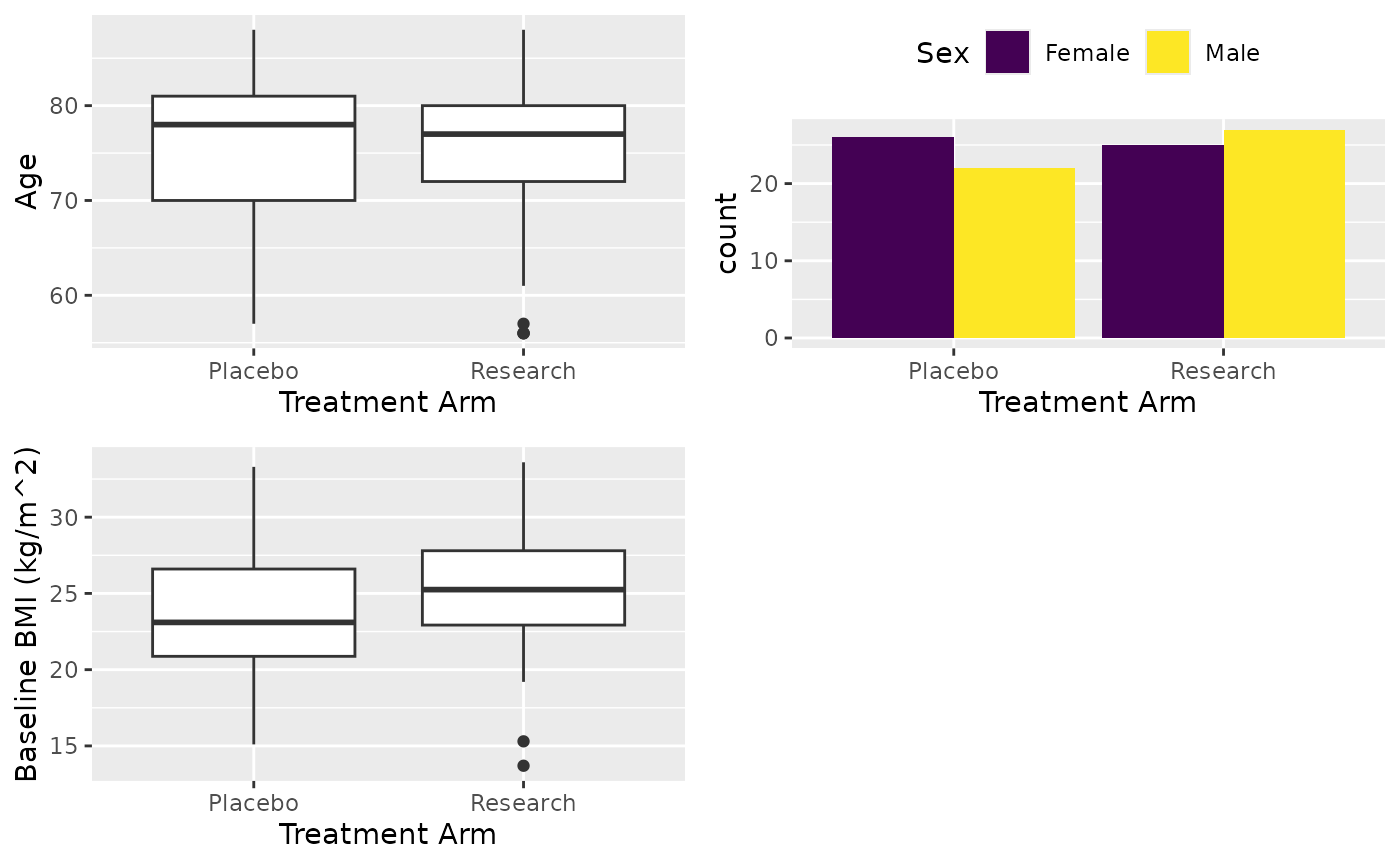


X
#> ┌───────────────────┬─────────────────┬──────────────────┬──────────────────┐
#> |                   │     Placebo     │     Research     │      Total       |
#> ├───────────────────┴─────────────────┴──────────────────┴──────────────────┤
#> |Observation        │       48        │        52        │       100        |
#> ├───────────────────┬─────────────────┬──────────────────┬──────────────────┤
#> ├───────────────────┴─────────────────┴──────────────────┴──────────────────┤
#> |Age                                                                        |
#> ├───────────────────┬─────────────────┬──────────────────┬──────────────────┤
#> |  Valid Obs.       │       48        │        52        │       100        |
#> |  Mean (SD)        │  75.52 (7.86)   │   74.75 (8.04)   │   75.12 (7.93)   |
#> |  Median [Min, Max]│   78 [57, 88]   │   77 [56, 88]    │   77 [56, 88]    |
#> ├───────────────────┴─────────────────┴──────────────────┴──────────────────┤
#> |Sex                                                                        |
#> ├───────────────────┬─────────────────┬──────────────────┬──────────────────┤
#> |  Female           │  26/48 (54.2%)  │  25/52 (48.1%)   │  51/100 (51.0%)  |
#> |  Male             │  22/48 (45.8%)  │  27/52 (51.9%)   │  49/100 (49.0%)  |
#> ├───────────────────┴─────────────────┴──────────────────┴──────────────────┤
#> |Baseline BMI (kg/m^2)                                                      |
#> ├───────────────────┬─────────────────┬──────────────────┬──────────────────┤
#> |  Valid Obs.       │       48        │        52        │       100        |
#> |  Mean (SD)        │  23.55 (4.05)   │   25.29 (4.1)    │   24.45 (4.15)   |
#> |  Median [Min, Max]│23.1 [15.1, 33.3]│25.25 [13.7, 33.6]│24.35 [13.7, 33.6]|
#> └───────────────────┴─────────────────┴──────────────────┴──────────────────┘

Alimu Dayimu

2025-11-06